Time-Varying Ensemble Detection
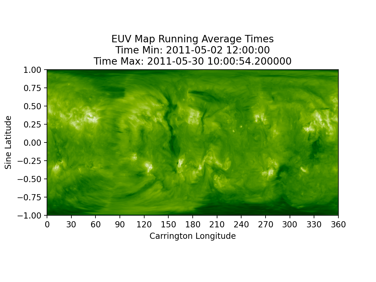
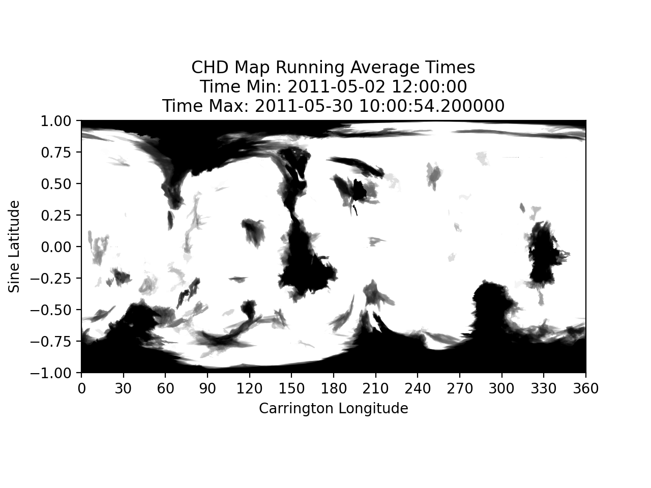
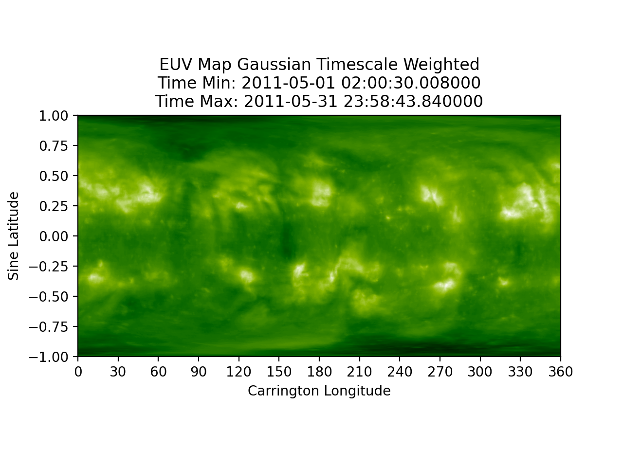
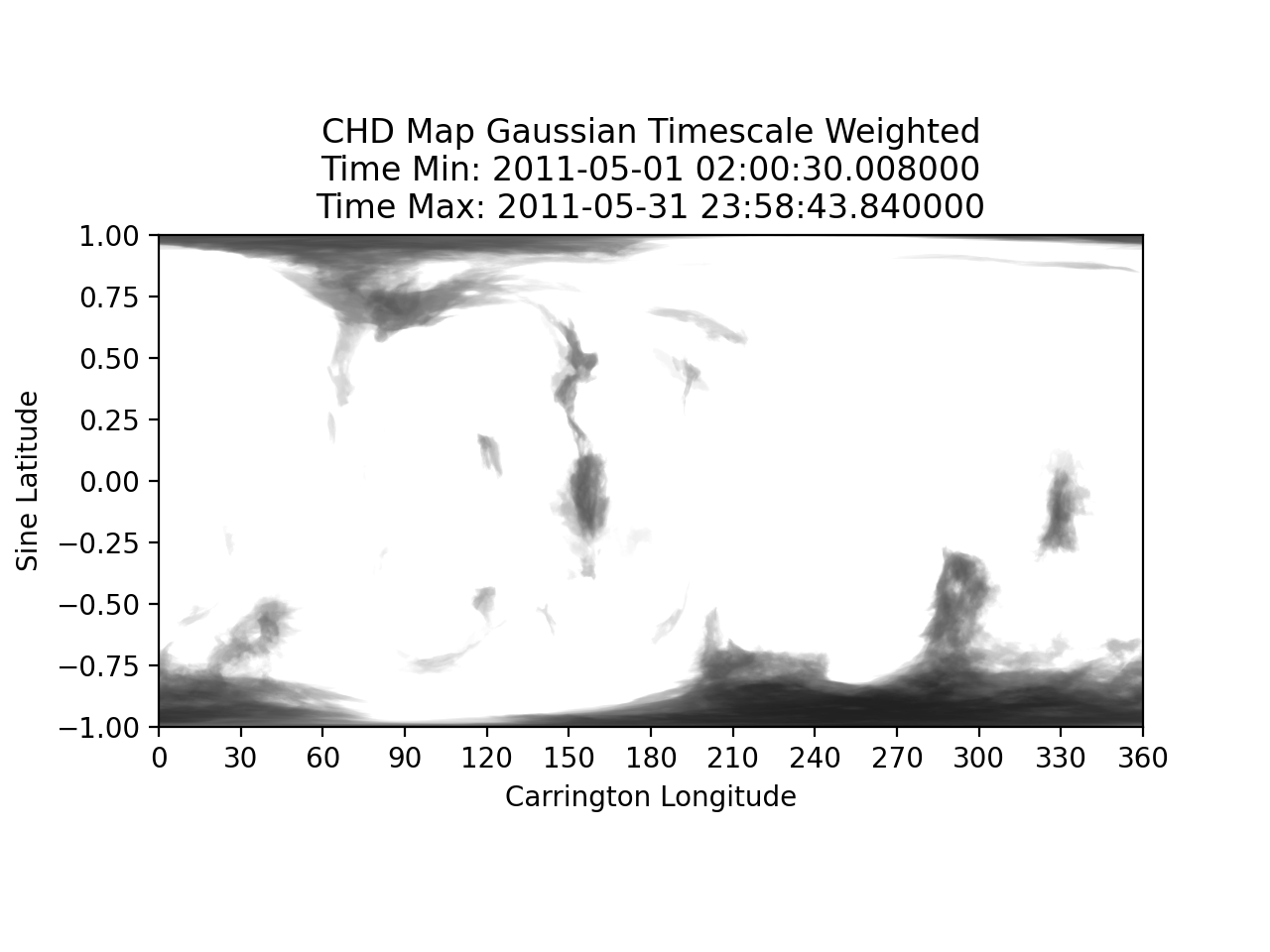
There are currently two methods of creating time-varying maps.
The first creates maps of varying timescale based on user entered intervals around a specific user inputted center date. These maps are then combined with a weighted average - either user inputted, or evenly weighted.
The code for running average maps is found here.
The second method uses a Gaussian distribution and a user inputted center date. The closer an image is to the center date, the more weight it has. Images are added one at a time to create the resultant maps.
The code for gaussian time weighted maps is found here.
Running Average Maps
| EUV Map | CHD Map |
|---|---|
 |
 |
Gaussian Time Varying Maps
| EUV Map | CHD Map |
|---|---|
 |
 |
Code Outline
Running Average Maps
This outline creates individual combined maps based on user defined timescales (1 day, 1 week, 2 weeks, etc.), then combines the maps based on user defined weighting.
1 2 3 4 5 6 7 8 9 10 11 12 13 14 15 | |
- 1.)
timescale_weight = [1.0 / len(timescales)] * len(timescales)- if the timescale weights are undefined, create an array of even weights
- 2.)
raise ValueError- check that the weights in the array add up to 1
- 3.)
chd_funcs.get_inst_combos- query the appropriate combo ids for each instrument based off the maximum time range the user inputted
- 4.)
db_funcs.query_euv_images- query the database for images based off the time range and center date
- 5.)
cr_funcs.apply_ipp- apply image pre-processing corrections
- 6.)
cr_funcs.chd- apply the Coronal Hole Detection algorithm to the image
- 7.)
cr_funcs.create_map- convert the image and detection to a map
- 8.)
cr_funcs.cr_map- create combined maps using the method for synoptic mapping
- 9.)
dp_funcs.create_timescale_maps- combine the timescale maps to create a running average map, based off the timescale combination function
- 10.)
dp_funcs.save_timescale_maps- plot and save timescale maps to the database, including the methods combination
Gaussian Time Varying Maps
This method first creates a gaussian distribution and then weights images based off their closeness to a center date.
1 2 3 4 5 6 7 8 | |
- 1.)
chd_funcs.get_inst_combos- query the appropriate combo ids for each instrument based off the maximum time range the user inputted
- 2.)
db_funcs.query_euv_images- query the database for images based off the time range and center date
- 3.)
dp_funcs.gauss_time- generate a gaussian distribution based off the number of images queried and user defined sigma balue
- 4.)
cr_funcs.apply_ipp- apply image pre-processing corrections
- 5.)
cr_funcs.chd- apply the Coronal Hole Detection algorithm to the image
- 6.)
cr_funcs.create_map- convert the image and detection to a map
- 6.)
dp_funcs.time_wgt_map- create combined maps based off the weighting of the Gaussian distribution
- 7.)
dp_funcs.save_gauss_time_maps- plot and save time weighted maps to the database, including the methods combination